MNIST Neural Nets

During my sophomore year of high school, I had a job working for an astrophysicist at Los Alamos National Laboratory. He has a completely free program for local teenagers interested in learning Python, which I had participated in several years prior. In my job, I wrote new chapters in the online textbook he used to teach it (he also makes this publicly availably). I wrote six chapters in the book, as well as overhauling another one. Unfortunately, most of the chapters were deemed too lengthy or complex to make the final cut of the book and now languish in an “incomplete chapter” section. This post will be about the most complex of these and the programs I wrote to illustrate the topic: neural networks.

I did a deep dive into both the math behind the neural networks (which I didn’t end up including in the chapters due to its complexity) and the programming skills necessary to implement it. I used the NetworkX library to represent the neural nets, which doesn’t have any built-in machine learning methods. This was all programmed by hand, and explained in a way hopefully parsable to a novice programmer.

I started with a very simple case: predicting polynomial data. As this was meant to be a gentle introduction to neural networks, I opted to use a genetic algorithm instead of backpropagation (which I’ll explain later). This meant starting with all of the parameters of the network in a random configuration and then tweaking them randomly over iterations until they produced an acceptably close fit to the data. This was a relatively simple endeavor, and the program and final result are shown below:

These are the helper functions, which are imported at the top of many of the programs shown below.

import networkx as nx
import numpy as np
import matplotlib.pyplot as plt
import random # for weights

def generate_blank_net(layer_sizes):
    """creates a network with a specified number of neurons in each layer and random weights."""
    blank_net = nx.DiGraph()
    for i in range(len(layer_sizes)):
        for j in range(layer_sizes[i]):
            neuron = f'l{i}_{j}' # properly formats the neuron names
            blank_net.add_node(neuron)
        blank_net.add_node(f'l{i}_b', activation=1)
    blank_net.remove_node(f'l{len(layer_sizes) - 1}_b') # remove bias neuron in output layer

    for n_1 in blank_net.nodes:
        n_1_layer = int(n_1.split('_')[0][1:])
        for n_2 in blank_net.nodes:
            # we need to check if the neurons are in adjacent layers, and make sure that the second neuron isn't a bias.
            n_2_layer = int(n_2.split('_')[0][1:])
            if n_1_layer + 1 == n_2_layer and n_2[-1] != 'b':
                blank_net.add_edge(n_1, n_2, weight=random.random()*2 - 1)
    
    return blank_net

def generate_layer_dict(net):
    """make a dictionary of a given neural net keyed by layer."""
    layer_dict = {}
    for neuron in net.nodes:
        neuron_layer = int(neuron.split('_')[0][1:]) 
        if neuron_layer not in layer_dict.keys():
            layer_dict[neuron_layer] = []
        layer_dict[neuron_layer].append(neuron)
    return layer_dict

def calc_next_layer(previous_layer_index, net, layer_dict, output=False):
    """given a neural net and the index of the last calculated layer, iterate the calculation one layer further."""
    for n_1 in layer_dict[previous_layer_index + 1]: # n_1 is the neuron that gets a new activation
        activation = 0
        if n_1[-1] != 'b':
            for n_2 in layer_dict[previous_layer_index]:
                activation += net.nodes[n_2]['activation'] * net[n_2][n_1]['weight']
            if output:
                net.nodes[n_1]['activation'] = activation
            else:
                net.nodes[n_1]['activation'] = np.tanh(activation)
        else:
            net.nodes[n_1]['activation'] = 1

    return net

def calc_all_layers(input_layer, net, layer_dict): 
    """returns the output layer given a neural net and an input layer."""
    if len(input_layer) != len(layer_dict[0]) - 1: # make sure the input layer is valid
        raise Exception(f'Input layer must be the same length as the first layer of nodes! (input is {input_layer} and first layer is {len(layer_dict[0]) - 1} long)')
    input_layer.append(1) # add bias neuron value
    for i in range(len(input_layer)):
        net.nodes[layer_dict[0][i]]['activation'] = input_layer[i]
    input_layer.pop(-1)

    for i in range(len(layer_dict) - 1):
        output = (i == len(layer_dict) - 2)
        net = calc_next_layer(i, net, layer_dict, output=output)

    output_layer_neurons = layer_dict[np.max(list(layer_dict.keys()))]
    output_layer_neurons.sort(key=lambda x: x.split('_')[1])
    output_layer = []
    for neuron in output_layer_neurons:
        output_layer.append(float(net.nodes[neuron]['activation']))
    
    return output_layer

This is the main genetic algorithm program.

from helper_functions import *

def main():
    poly_coeffs = [0.4, -1, 1, 1]
    domain = [-2,1.5]
    num_points = 100
    noise = 0.6
    num_children_per_net = 50
    num_survive = 5
    variance = 0.1
    generations = 150
    net_dimensions = [1,5,5,5,1]
    
    first_parent = generate_blank_net(net_dimensions)
    xs, ys = generate_polynomial_data(poly_coeffs, domain, num_points, noise)
    next_gen = make_next_gen([first_parent], xs, ys, num_children_per_net, num_survive, variance) # create first generation
    
    inputs = []
    expected_outputs = []
    for i in range(len(xs)):
        inputs.append(xs[i][0])
        expected_outputs.append(ys[i][0])  # reformat xs and ys for matplotlib
    
    for i in range(generations):
        next_gen = make_next_gen(next_gen, xs, ys, num_children_per_net, num_survive, variance)
        print(f'The RSS is {eval_total_cost(next_gen[0], xs, ys) * 1000} after generation {i+1}.') # the times 1000 makes the RSSs a reasonable value
        
        outputs = []
        for i in range(len(xs)):
            outputs.append(calc_all_layers(xs[i], next_gen[0], generate_layer_dict(next_gen[0])))
        plt.clf()
        plt.plot(inputs, expected_outputs)
        plt.plot(inputs, outputs)
        plt.savefig('fitted-curve.png')
        print('Figure saved to fitted-curve.png')          

def eval_RSS(net_outputs, expected_outputs):
    """gets RSS for a given set of outputs"""
    RSS = 0
    for i in range(len(net_outputs)):
        for j in range(len(net_outputs[i])):
            RSS += ((net_outputs[i][j] - expected_outputs[i][j]) ** 2) / len(net_outputs[i]) # make error independant of output layer size
    RSS /= len(net_outputs) # make error independant of data set size
    return RSS

def eval_total_cost(net, input_layers, expected_output_layers):
    """properply formats inputs to eval_RSS"""
    net_outputs = []
    layer_dict = generate_layer_dict(net)
    for i in range(len(input_layers)):
        net_outputs.append(calc_all_layers(input_layers[i], net, layer_dict))
    cost = eval_RSS(net_outputs, expected_output_layers)
    return cost / len(input_layers)
                       
def make_children(net, variance, num_children):
    """creates a specificied number of tweaked copies of a given net"""
    children = []
    for i in range(num_children):
        child = nx.DiGraph(net)
        for edge in child.edges:
            child.edges[edge]['weight'] += random.random() * variance - variance / 2
        children.append(child)
    return children

def make_next_gen(parents, input_layers, expected_output_layers, num_children_per_net=20, num_survive=1, variance=0.1):
    """creates many of copies of a net, tweaks them slightly, then picks out the best ones to create the next generation."""
    children = parents.copy() # make sure RSS doesn't go up
    best_children = []
    costs = []
    for parent in parents:
        loop_children = make_children(parent, variance, num_children_per_net)
        for child in loop_children:
            children.append(child)
    for child in children:
        costs.append(eval_total_cost(child, input_layers, expected_output_layers))
        
    for i in range(num_survive):
        best_child_index = costs.index(np.min(costs))
        best_children.append(children[best_child_index])
        children.pop(best_child_index)
        costs.pop(best_child_index)

    return best_children
                                 
def generate_polynomial_data(coefficients, domain, num_points, noise=0):
    """returns two formatted lists: one for inputs, the other for expected outputs"""
    xs = np.linspace(domain[0], domain[1], num_points)
    ys = []
    xs_lists = [] # because of numpy syntax, we have to make two xs arrays
    for i in range(len(xs)):
        # add variation to the data to give fitting a thourough test
        xs[i] += random.random() * (domain[1] - domain[0]) * noise / (0.1 * num_points) - (domain[1] - domain[0]) * noise / (0.2 * num_points)
        xs_lists.append([xs[i]])
        # input_layers is a list of lists, so this formats the inputs properly
        y = 0
        for j in range(len(coefficients)):
            y += (coefficients[j] * (xs[i] ** j)) + (random.random() * noise) - (noise / 2)
        ys.append([y]) # same as above but for outputs
    return xs_lists, ys

if __name__ == '__main__':
  main()

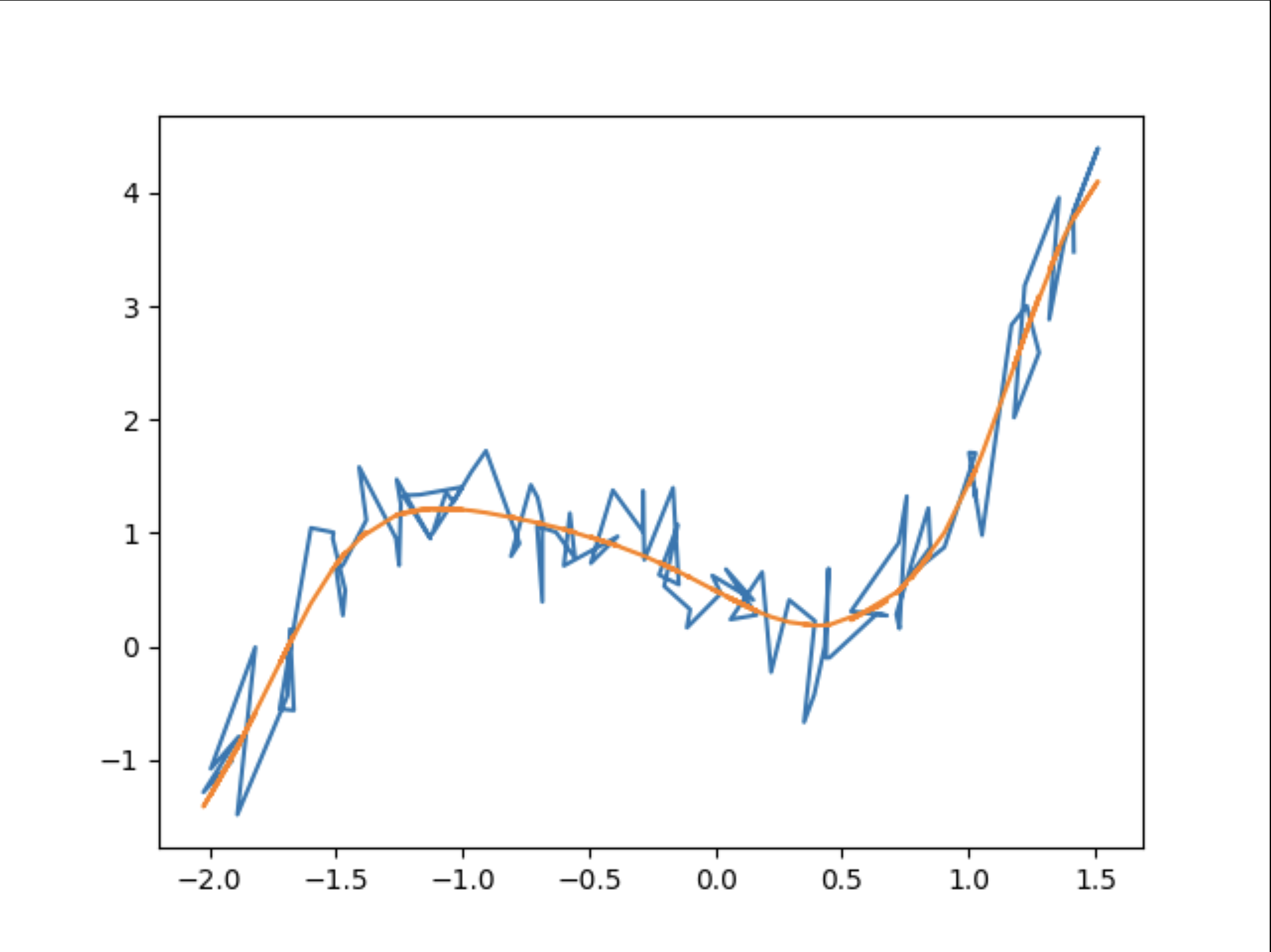
This method produces a very good fit of the data, especially considering how noisy it is. The next application of this was to use it on a real data set (which I chose to be used car data), which produced similar well-fitting results. However, my main goal in this project was not to have a roundabout way of fitting data. So, I wrote another section of the neural network chapter in the book, this time about backpropagation. I spent much more time on this section, both in the programming and in the writing itself. It is definitely one of the most complex programming tasks I have attempted, making it a rewarding and challenging experience.

In the new section, I introduced the idea of a Python class. I used it heavily throughout the chapter, sometimes in places that it may not strictly be the best idea, but I felt it was a good way to show the various use cases it can have. The data that I fitted with my program is the Modified National Institute of Standards and Technology (MNIST) dataset. This data catalogs tens of thousands of handwritten digits in a 28x28 pixel format. This large amount of data combined with small computation power required for each individual image made it ideal for my purposes.

This is the main body of the MNIST training program, which will be explained in more detail below.

import numpy as np
import struct
from array import array
import random
import matplotlib.pyplot as plt

class MnistDataloader(object):
    def __init__(self, training_images_filepath,training_labels_filepath, test_images_filepath, test_labels_filepath):
        self.training_images_filepath = training_images_filepath
        self.training_labels_filepath = training_labels_filepath
        self.test_images_filepath = test_images_filepath
        self.test_labels_filepath = test_labels_filepath
    
    def read_images_labels(self, images_filepath, labels_filepath):
        """processes data and converts images and labels to arrays"""
        with open(labels_filepath, 'rb') as file:
            size = struct.unpack(">II", file.read(8))[1]
            unformatted_labels = array("B", file.read())
            labels = np.zeros((len(unformatted_labels), 10))
            for i in range(len(labels)):
                labels[i][unformatted_labels[i]] = 1.0
        
        with open(images_filepath, 'rb') as file:
            size, rows, cols = struct.unpack(">IIII", file.read(16))[1:]
            image_data = array("B", file.read())        
        images = np.zeros((size, rows * cols))
        for i in range(size):
            images[i] = np.array(image_data[i * rows * cols:(i + 1) * rows * cols]) / 256            
        
        return images, labels
            
    def load_data(self):
        """returns processed data for both training and testing"""
        x_train, y_train = self.read_images_labels(self.training_images_filepath, self.training_labels_filepath)
        x_test, y_test = self.read_images_labels(self.test_images_filepath, self.test_labels_filepath)
        return x_train, y_train, x_test, y_test     

class layer():
    """A fully connected layer with forward and backward propagation"""
    def __init__(self, input_size, output_size):
        self.type = 'layer'
        self.weights = np.random.randn(input_size, output_size)
        self.biases = np.zeros((1, output_size))
        self.params = [self.weights, self.biases]

    def prop_forward(self, inputs):
        self.inputs = np.array(inputs)
        self.outputs = np.dot(self.inputs, self.weights) + self.biases
        return self.outputs

    def prop_backward(self, next_grad):
        self.weight_grad = np.dot(self.inputs.T, next_grad)
        self.bias_grad = np.sum(next_grad, axis=0)
        self.next_grad = np.dot(next_grad, self.weights.T)
        return self.next_grad        

class sigmoid():
    """the sigmoid activation function"""
    def __init__(self):
        self.type = 'func'
        # for when we update weights
        self.weights = None
        self.biases = None
        self.params = [None, None]
    
    def prop_forward(self, inputs):
        self.inputs = inputs
        self.outputs = 1/(1 + np.exp(-inputs))
        return self.outputs

    def prop_backward(self, next_grad):
        self.weight_grad = [None]
        self.bias_grad = [None]
        self.next_grad = next_grad * (1 - next_grad)
        return self.next_grad / len(next_grad)
    
class NN():
    """A neural network class based on layer and activation function classes"""
    ## all inputs in a batch are processed simultaneously in this model.
    ## this means many arrays in this have batch size as the first entry
    ## in their shape.
    def __init__(self):
        self.layers = []
        self.params = []

    def add_layer(self, layer):
        """adds a layer to the net"""
        self.layers.append(layer)
        self.params.append(layer.params)

    def remove_layer(self, index):
        """removes a layer from the net"""
        self.layers.pop(index)
        self.params.pop(index)

    def run_forward(self, inputs):
        """runs inputs through the net and updates output values"""
        self.activations = inputs.copy()
        for layer in self.layers:
            self.activations = layer.prop_forward(self.activations)
        self.outputs = self.activations.copy()
    
    def run_backward(self, next_grad):
        """runs errors through the net and update gradients"""
        self.grads = []
        for layer in reversed(self.layers):
            next_grad = layer.prop_backward(next_grad)
            self.grads.append([layer.weight_grad, layer.bias_grad])

    def update_params(self, inputs, expected_outputs, l_rate, v_depreciate):
        """updates weights and biases based on gradients"""
        self.run_forward(inputs)
        output_error = self.outputs - expected_outputs
        self.run_backward(output_error)

        layer = 0
        for p, g, v in zip(self.params, reversed(self.grads), self.velocities):
            # some of these will be filled with None due to ReLU layers
            if self.layers[layer].type == 'layer':
                for i in range(len(g)):
                    g[i] = np.array(g[i], dtype=float)# g can be an array of integers, which is changed to floats
                    v[i] = v_depreciate * v[i] + g[i]
                    p[i] -= l_rate * v[i]
                    if i == 0: # checks to see whether p is weights or biases
                        self.layers[layer].weight = p[i]
                    else:
                        self.layers[layer].biases = p[i]
                self.layers[layer].params = p

            layer += 1

    def generate_batch(self, xs, ys, batch_size):
        """returns a random sample of the given data"""
        batch_xs = []
        batch_ys = []
        shuffle = np.random.permutation(len(xs))
        xs, ys = xs[shuffle], ys[shuffle]
        for i in range(batch_size):
            batch_xs.append(xs[i])
            batch_ys.append(ys[i])
        return batch_xs, batch_ys

    def calc_accuracy(self, expected_outputs):
        """returns the accuracy of the net after calculating the output"""
        accuracy = 0
        maxxes = np.amax(self.outputs, axis=1)
        for i in range(len(expected_outputs)):
            if np.where(self.outputs[i] == np.max(self.outputs[i]))[0] == np.where(expected_outputs[i] == 1.0)[0]:
                accuracy += 100 / len(expected_outputs)
        
        return accuracy
    
    def train(self, epochs, inputs, expected_outputs, batch_size, learning_rate=0.1, velocity_depreciation=0.9, real_time=True):
        """trains the net with the specified hyperparameters"""
        self.velocities = []
        for param_layer in self.params: 
            self.velocities.append([np.zeros_like(param) for param in param_layer])

        accuracies = []
        for i in range(epochs):
            batch_inputs, batch_expected_outputs = self.generate_batch(inputs, expected_outputs, batch_size)
            self.update_params(batch_inputs, batch_expected_outputs, learning_rate, velocity_depreciation)
            accuracy = self.calc_accuracy(batch_expected_outputs)
            print(f'Epoch {i+1} ran succesfully. Accuracy: {round(accuracy, 6)}')
            accuracies.append(accuracy)
            if real_time:
                plt.plot(range(len(accuracies)), accuracies)
                plt.savefig('real_time_accuracy.png')
                print('Accuracy graph saved to real_time_accuracy.png')
                plt.clf()
        
        print(f'Training complete.')
        return accuracies # for graphing accuracies over epochs

    def test(self, test_inputs, test_expected_outputs):
        """tests the net with the provided data"""
        self.run_forward(test_inputs)
        accuracy = self.calc_accuracy(test_expected_outputs)
        print(f'Test complete. Accuracy: {round(accuracy, 6)}')
        return accuracy

def main():
    shape = [784, 32, 10]
    activation_func = sigmoid
    learning_rate = 1
    velocity_depreciation = 0.9
    epochs = 150
    batch_size = 250
    
    filepaths = ['train-images.idx3-ubyte','train-labels.idx1-ubyte','t10k-images.idx3-ubyte','t10k-labels.idx1-ubyte']
    
    inputs, expected_outputs, test_inputs, expected_test_outputs = MnistDataloader(filepaths[0], filepaths[1], filepaths[2], filepaths[3]).load_data()
    
    net = NN()
    for i in range(len(shape) - 1):
        net.add_layer(layer(shape[i], shape[i+1]))
        net.add_layer(activation_func())
        
    accuracies = net.train(epochs, inputs, expected_outputs, batch_size, learning_rate, velocity_depreciation, real_time=False)
    test_accuracy = net.test(test_inputs, expected_test_outputs)
    
    plt.plot(range(epochs), accuracies)
    plt.show()
    
if __name__ == '__main__':
  main()

This is, obviously, a very lengthy program. The main idea of it, though, can be found from basic calculus. Backpropagation is just a fancy word for gradient descent, albeit in a very high-dimensional space. To calculate the gradient, one has to calculate the derivative of each parameter (that is, weights and biases for each neuron) with respect to the value to be minimized, which is the error at the output. This can be done by repeated applications of the chain rule backward through the net (hence the name backpropagation), as is explained below.

First, imagine a net with no activation function. This means each neuron activation is the weighted sum of the previous layer with no extra processing. As this is a simple case, the math will be easier to understand, which can be built upon later. Consider a given neuron in the layer before the output. To understand how this could be tweaked to improve the accuracy of the net, we need two things: the weights that connect this neuron to the output, and the activation of the neuron. With these, it’s trivial to calculate $\frac{\partial w_{ij}}{\partial L}$, where $w_{ij}$ is a given weight between neurons $i$ and $j$ in adjacent layers and $L$ is the loss, or total error in the output. This is just an algebraic operation, as it’s obvious how changing each weight would affect the output. The true power of backpropagation comes from the next step, however. The other set of derivatives needed are all $\frac{\partial a_i}{\partial L}$, where $a_i$ is the activation of neuron $i$. Now that we know how each neuron in that layer should change, we can repeat the process the exact same way for the next layer. That leaves us with $\frac{\partial b_j}{\partial a_i}$, where $b_i$ is the activation for the new layer we’re operating on. If we then multiply all of these by the corresponding $\frac{\partial a_i}{\partial L}$, giving us $\frac{\partial b_j}{\partial L}$. These absolute activation derivatives allow us to calculate the gradient for all weights (and biases) in the net.

If we add an activation function $A(b_{j_0} w_{j_0i} + b_{j_1} w_{j_1i} + …)$, the only thing that changes is that we need to add another chain rule step when moving from one layer to the previous. By multiplying by the derivative of the inverse of the activation function, this happens automatically. This is easily illustrated by the following:

\[\begin{align*} A(b_{j_0} w_{j_0i} + b_{j_1} w_{j_1i} + ...) &= a_i \\ b_{j_0} w_{j_0i} + b_{j_1} w_{j_1i} + ... &= A^{-1}(a_i)\\ w_{j_0i}\frac{\partial b_{j_0}}{\partial L} + w_{j_1i}\frac{\partial b_{j_1}}{\partial L} + ... &= \frac{\partial A^{-1}(a_i)}{\partial a_i} \frac{\partial a_i}{\partial L} \end{align*}\]

If we set all other activation derivatives to zero, we can then solve for each individual derivative. These activation derivatives can then be used to calculate the weight derivatives and update the entire net. In practice, this can be done for many, many inputs at once in parallel, using matrix multiplication. This is how my implementation listed above runs, using the NumPy library.

None of this math ended up in the chapter I wrote because it was simply too advanced for the intended audience. However, to get the program to function, I did have to learn it all, so I felt it was fitting to include it here.

TKInter inputs:

The next major step I took was to make the program interactive. After all, it’s not an incredibly helpful educational tool if it just displays a message that says “test accuracy: 98.2%” or something like that. In order to make it interactive, though, I had to familiarize myself with yet another Python library: TKInter. It’s a GUI library, which has applications in any scenario where a display window is required. Unfortunately, unlike MatPlotLib (which I had previously been using to graph accuracy, etc.), it doesn’t have built-in compatibility with NetworkX. This meant I had to interface them manually, which took a lot of effort and consideration of exact pixel locations. The updated sections of the code are below:

The new code required for interactions.

""" add this line at the top: """
import tkinter as tk

""" replace the last two lines of main with: """
    for _ in range(10):
        i = random.randint(0, len(inputs) - 1)
        image = inputs[i]
        label = expected_outputs[i]
        net.run_forward([image])
        output = net.outputs[0]
        show_example(image, list(output).index(np.max(output)), list(label).index(1))

    pad = DrawPad(net.run_forward) ## creates a drawing pad that will run the output through the trained net
    while pad.root.state() == 'normal': # checks if the window tkinter opened is still open 
        pad.get_input() ## automatically runs output through net
        print(f'Net output: {list(net.outputs[0]).index(np.max(net.outputs[0]))}')

def show_example(image, net_output, expected_output):
    """shows an image, the net output, and the image's label"""
    root = tk.Tk()
    root.title('Digit')
    canvas = tk.Canvas(root, width=560, height=560, bg='black')
    canvas.pack()
    image = image.reshape(28, 28).T
    for x in range(image.shape[0]):
        for y in range(image.shape[1]):
            pix_val = image[x][y] * 255
            fill = rgb_hex((pix_val, pix_val, pix_val))
            canvas.create_rectangle(x * 20 - 10, y * 20 - 10, x * 20 + 10, y * 20 + 10, fill=fill, width=0)
    print(f'Net output: {net_output}')
    print(f'Label: {expected_output}')
    root.mainloop()

def rgb_hex(rgb):
    """turns an rgb color into a hexcode color"""
    r, g, b = rgb
    return f'#{int(r):02x}{int(g):02x}{int(b):02x}'

""" add this class somewhere in the body: """
class DrawPad():
    def __init__(self, output_command):
        """sets up various necessary variables"""
        self.output_command = output_command
        self.root = tk.Tk()
        self.pixels = np.zeros((28, 28))
        self.root.title('Input Digit:')
        self.root.minsize(560, 600)
        self.canvas = tk.Canvas(self.root, width=560, height=560, bg='black')
        self.canvas.pack()
        self.canvas.bind('<B1-Motion>', self.draw_pixels) # B1-Motion is when the left-click is held and dragged
        self.frame = tk.Frame(self.root)
        self.frame.pack(side=tk.BOTTOM)
        tk.Button(self.frame, text='Submit', font='comicsans 12 bold', command=self.output).pack(side=tk.BOTTOM, padx=6, pady=6)
        tk.Button(self.frame, text='Clear', font='comicsans 12 bold', command=self.clear).pack(side=tk.BOTTOM, padx=6)

    def draw_pixels(self, mouse):
        """draws a 3x3 diamond of pixels around the cursor"""
        # snaps xs and ys to a 28x28 grid
        x = np.floor(mouse.x / 20) * 20 + 10
        y = np.floor(mouse.y / 20) * 20 + 10
        for dx in range(-40, 60, 20):
            for dy in range(-40, 60, 20):
                if not ((abs(dx) == 40 and abs(dy) == 40) or (abs(dx) == 20 and abs(dy) == 40) or (abs(dx) == 40 and abs(dy) == 20)):
                    # selects a diamond-shaped region around the mouse
                    if abs(dx) == 20 or abs(dy) == 20:
                        # selects four pixels adjacent to center
                        dalpha = 10 / 255
                    elif abs(dx) == 40 or abs(dy) == 40 or (abs(dx) == 20 and abs(dy) == 20):
                        # selects 8 pixels not adjacent to center
                        dalpha = 3 / 255
                    else:
                        # selects center pixel
                        dalpha = 80 / 255
                    self.pixels[int((x + dx - 10) / 20)][int((y + dy - 10) / 20)] += dalpha # increases the value of a pixel
                    if self.pixels[int((x + dx - 10) / 20)][int((y + dy - 10) / 20)] > 1:
                        self.pixels[int((x + dx - 10) / 20)][int((y + dy - 10) / 20)] = 1
                    self.draw_rec((x - 10 + dx, y - 10 + dy), (x + 10 + dx, y + 10 + dy), alpha=self.pixels[int((x + dx - 10) / 20)][int((y + dy - 10) / 20)] * 255)

    def rgb_hex(self, rgb):
        """turns an rgb color into a hexcode color"""
        r, g, b = rgb
        return f'#{int(r):02x}{int(g):02x}{int(b):02x}'
                    
    def draw_rec(self, pt_1, pt_2, alpha=255):
        """draws a given pixel at a given alpha"""
        fill = self.rgb_hex((alpha, alpha, alpha))
        self.canvas.create_rectangle(pt_1[0], pt_1[1], pt_2[0], pt_2[1], fill=fill, width=0)

    def clear(self):
        """clears the canvas"""
        self.canvas.delete('all')
        self.pixels = np.zeros((28, 28))

    def output(self):
        """outputs the current state of the canvas"""
        self.output_command(self.pixels.T.reshape(1, 784))
        self.root.quit()
        
    def get_input(self):
        """displays the canvas and buttons"""
        self.root.mainloop()

This is a very bare-bones UI, though it easily could be expanded to include more features. An example digit drawn with it is pictured below:

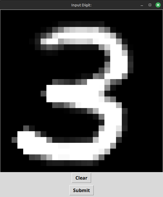
When ‘Submit’ was clicked, the window closed, and the net’s output was printed to the console. It would also draw 10 (an arbitrarily chosen number) example digits before displaying the drawing pad to give the user examples of what digits should look like. If the style was wrong, the net would misidentify it, as it had only been trained on the specific style found in the MNIST data.

Conclusion:

This project was very far-reaching and pushed the boundaries of what I knew in many fields. It was incredibly frustrating at times, but ultimately I pushed through and now have a better and more intuitive understanding of neural networks, multivariable calculus, the TKInter, NetworkX, and NumPy libraries, and Python classes. This is one of the projects I’m most proud of, and I hope to find more like it in the future.