Kepler Ptolemy Simulation

This is a subsection of my Kepler Ptolemy project, in the math section. This is a big part of what I worked on in that project, but I felt it was more fitting in the programming section. This will be a shorter description, but it still taught me some valuable things.

What inspired this project was simply a desire to see what the Kepler Ptolemy system could look like when we eventually solved the system of differential equations. Cris (Cristopher Moore, who was my mentor for the larger Kepler Ptolemy project) delegated it to me, as it’s relatively simple and I’m familiar enough with Python to do it easily (or so I thought). My initial approach was to choose some angle step from the equant, then step out along that line until the area swept out by the most recent step is equal to our initial area step (this ensures that angular momentum is conserved, as discussed in the main post):

import matplotlib.pyplot as plt
import numpy as np
import math

def main():

    final_angle = np.pi
    angle_step = 0.001 * np.pi
    distance_step = 0.0001

    r = np.array((2, 0))
    new_r = r + (0, math.sin(angle_step) * mag(r))

    l = np.array((1, 0))
    fig, ax = plt.subplots(1, 1)
    ax.plot((0, l[0]), (0, l[1]), 'o', color='grey')
    semi_perim = 0.5 * (mag(r - l) + mag(r - new_r) + mag(new_r - l))
    area_step = math.sqrt(semi_perim * (semi_perim - mag(r - l)) * (semi_perim - mag(r - new_r)) * (semi_perim - mag(new_r - l)))
    print(area_step)

    points = [r]
    for i in np.arange(0, final_angle, angle_step):
        ## update and record the position
        r = step(r, l, angle_step, area_step, distance_step)
        points.append(r)
    
    points = np.array(points)
    ax.plot(points[:, 0], points[:, 1])
        
    plt.show()
    
def step(r, l, angle_step, area_step, distance_step):
    ## uses the geometry of a single step to determine the length of the next radius
    pol_r = [mag(r), math.acos(r[0] / mag(r))]
    if r[1] < 0: ## adjust range of acos properly
        pol_r[1] = 2 * np.pi - pol_r[1]
    
    calc_area = 0
    pol_new_r = np.array([0, pol_r[1] + angle_step])
    len_base = mag(r - l)
    while calc_area < area_step:
        pol_new_r[0] += distance_step
        new_r = polar_to_cart(pol_new_r)
        len_short_side = mag(new_r - r)
        len_long_side = mag(new_r - l)
        semi_perim = 0.5 * (len_base + len_short_side + len_long_side)
        calc_area = math.sqrt(semi_perim * 
                             (semi_perim - len_base) *
                             (semi_perim - len_short_side) *
                             (semi_perim - len_long_side)) ## Heron's formula
        print(calc_area)
        
    return new_r

def mag(vec):
    ## returns the magnitutde of a vector
    return math.sqrt(vec[0] ** 2 + vec[1] ** 2)
    
def angle(vec):
    ## returns the angle of a vector
    if mag(vec) == 0:
        return 0

    angle = math.acos(vec[0] / mag(vec))
    if vec[1] < 0:
        ## adjust range of acos
        angle = 2 * np.pi - angle
    return angle

def polar_to_cart(point):
    ## converts a point from polar to cartesian coordinates
    r, theta = point
    x, y = r*math.cos(theta), r*math.sin(theta)
    return np.array((x, y))

if __name__ == '__main__':
    main()

This method ultimately turned out to be unfruitful: If one were to run the above code, it would produce a mess of lines radiating from the equant. This is due to errors from starting the trawl along the radial line at length zero. To solve this issue, I found studying the geometry of a single timestep dt to be helpful:

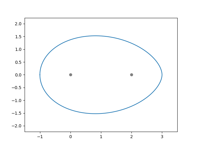
From this, it is apparent that there is an easily calculable point close to but not past the new position of the curve: where the two lines cross in the center of the diagram. Updating my step function in the above program to start at this new point, it began producing viable images:

However, I quickly realized something about this entire geometry: If I kept track of the velocity at all times (by subtracting the new position from the old one and dividing by the timestep), I could avoid any type of for loop in each individual timestep, which turned out to be very simple to implement. The final version of the program is below:

import matplotlib.pyplot as plt
import numpy as np
import math

def main():

    final_angle = 2 * np.pi 
    angle_step = 0.001 * np.pi ## can be set to improve resolution; however, higher resolution causes EARLIER divergence
    num_derivs = 0 ## number of derivatives to take and graph. 0 for only avocado
    
    ## initial position and velocity. Current conditions are good for producing stable avocados
    r = np.array((-1, 0))
    v = np.array((0, -1))
    
    ## only valid when r = -1, 0 and v = 0, -1
    ellipse = False ## display an ellipse of the given eccentricity on top of the avocado
    e = 0.5 ## eccentricity

    ### NON ADJUSTABLE THINGS ###

    l = (2 * e * mag(r) / (1 - e), 0)
    fig, ax = plt.subplots(1, 1)
    ax.plot((0, l[0]), (0, l[1]), 'o', color='grey')
    area_step = 0.5 * angle_step * mag(v) * mag(r - l) * math.sin(angle(v) - angle(r - l))

    ### ELLIPSE ###
    a = mag(l)/2 + mag(r)
    ell_points = []
    for i in np.arange(0, final_angle, angle_step):
        ## calculate an equivalent set of points to the avocado curve for the ellipse
        ell_r = (a * (1 - e ** 2)) / (1 - e * math.cos(i - angle(l) + np.pi))
        ell_points.append(polar_to_cart((ell_r, i + np.pi)))
    ell_points = np.array(ell_points)
    ## give graph reasonable constraints to prevent asmptotes from dominating
    ax.set_xlim(min(ell_points[:, 0]) - 0.5, max(ell_points[:, 0]) + 0.5)
    ax.set_ylim(min(ell_points[:, 1]) - 0.5, max(ell_points[:, 1]) + 0.5)
    if ellipse:
        ax.plot(ell_points[:, 0], ell_points[:, 1], color='orange')
        
    ### AVOCADO ###
    points = [r]
    for i in np.arange(0, final_angle, angle_step):
        ## update and record the position
        r = step(r, l, angle_step, area_step)
        points.append(r)
    
    points = np.array(points)
    ax.plot(points[:, 0], points[:, 1])
        
    plt.show()
    
    ### DERIVATIVES ###
    if num_derivs: ## do nothing if num_derivs is 0
        num_derivs += 1
        derivs = []
        for i in range(len(points)):
            new_set = []
            for j in range(num_derivs):
                new_set.append(take_deriv(points, i, j, angle_step))
            derivs.append(new_set)
            
        derivs = np.array(derivs[:-1 * num_derivs]) ## cut out edge derivs
        fig, axs = plt.subplots(1, num_derivs)
        for i, ax in enumerate(axs):
            ax.plot(derivs[:, i, 0], derivs[:, i, 1])
        plt.show()
    
def step(r, l, angle_step, area_step):
    ## uses the geometry of a single step to determine the length of the next radius
    radii_angle = angle(r - l) - angle(r)
    new_r = ((mag(r) * math.sin(radii_angle) - (2 * area_step / mag(r - l))) / math.sin(radii_angle - angle_step), angle(r) + angle_step)
    return polar_to_cart(new_r)
 
def mag(vec):
    ## returns the magnitutde of a vector
    return math.sqrt(vec[0] ** 2 + vec[1] ** 2)
    
def angle(vec):
    ## returns the angle of a vector
    if mag(vec) == 0:
        return 0

    angle = math.acos(vec[0] / mag(vec))
    if vec[1] < 0:
        ## adjust range of acos
        angle = 2 * np.pi - angle
    return angle

def polar_to_cart(point):
    ## converts a point from polar to cartesian coordinates
    r, theta = point
    x, y = r*math.cos(theta), r*math.sin(theta)
    return np.array((x, y))
    
def comb(n, r):
    ## n choose r
    return math.factorial(n) / (math.factorial(r) * math.factorial(n - r))

def take_deriv(points, i, d, time_step):
    ## approximate the dth derivative of points
    deriv = 0
    for j in range(d + 1):
       deriv += comb(d, j) * (-1) ** j * points[(i + j) % len(points)]
    deriv /= time_step ** d
    return list(deriv)

if __name__ == '__main__':
    main()

This version has several additional bells and whistles when compared to the first program, but the underlying idea is the same. This also allows the user to input the desired shape of curve as an “eccentricty,” much the same as an ellipse’s eccentricity. This also shows that the Kepler Ptolemy curves are indeed a one-parameter family, meaning every shape the closed form can take can be characterized by a single number.

This project, although summarized quickly in this post, took a lot of effort and debugging on my part. I learned some overarching programming concepts, such as looking for a more efficient representation of the problem and new debugging techniques, as well as more specific elements relevant to this problem, such as the one-parameter nature of the Kepler Ptolemy curves.