Kepler Ptolmey System

This project has spanned over a year and will culminate in the publication of an academic paper in a scientific journal. The subject matter is highly arcane and theoretical, but it has been highly instructive in a variety of areas of mathematics. I am working on this project under the mentorship of Professor Cristopher Moore, a researcher at the Santa Fe Institute.

Setup:

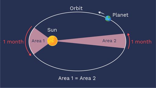
To outline what this project accomplished, I must first discuss certain properties of ellipses, specifically those traced out by one body orbiting another in Newtonian mechanics. In this, angular momentum is conserved from the perspective of the star (which sits at one of the foci), which is an equivalent statement to saying the planet sweeps out equal arcs of area in equal time, as seen in the diagram below.

Another seemingly interesting property of this ellipse is that from the other focus (called the empty focus, because there’s nothing there in a regular orbit) the planet almost conserves its angular speed. This means, standing at that point, the planet would sweep out very close to equal arcs of the sky per unit time.

Proving that in and of itself involved a non-trivial amount of work. I learned to use Mathematica, a software that can be extremely helpful for any sort of complex mathematics. I also gained a much more thorough understanding of variance, which is what we used to quantify the error from a uniform angular speed. As it turned out, the variance was proportional to a forth-order term in the eccentricity of the ellipse, ε. As such, for low eccentricities, uniform angular speed is a very good approximation.

The main problem we addressed, however, was finding a curve that exactly satisfies both the constant angular speed from one focus (which is just what we called them due to their correspondence to the foci of an ellipse - it doesn’t have any of the other properties of ellipse foci) and constant angular momentum from the other. We called these foci the equant and the sun respectively, as the first has the properties of Ptolemy’s equant, and the second has similar properties to the point at which more massive bodies sit in orbits.

Main problem:

To address this problem, it needs to be rephrased. The terminology used will be as follows:

• $\vec{r}$ is the radius from the empty focus to the planet
• $\vec{v}$ is the velocity of the planet
• $\theta$ is the angle of the planet from the empty focus
• $(x, y)$ are the cartesian coordinates of the planet, treating the empty focus as the origin
• $\ell$ is the distance between the foci
• $\vec{r}_\odot = \vec{r} - \vec{\ell}$ is the radius from the sun to the planet
• $\theta_\odot$ is the angle of the planet from the sun
• $\omega$ is the angular speed around the empty focus
• $J$ is the angular momentum around the sun focus

Now, the two conditions can be specified:

\[\text{Angular speed: }\omega = \frac{\vec{r} \times \vec{v}}{r^2} \\ \text{Angular momentum: }J = \vec{r}_\odot \times \vec{v}\]

From these, we learned several things. Most importantly, $y’ = \frac{\omega r^2 - J}{\ell} $, which we used later as a basis for substitution and conversion to polar coordinates. I won’t go into all the details (I’ll attach a copy of the paper at the bottom which has everything laid out explicitly), but this system of differential equations turns out to be closely related to the Legendre polynomials, which lead to various families of solutions in a process outlined in a later section.

My main independent contributions to this project were in the form of small details that needed proving. For instance, we observed in simulations (which I’ve written about coding here) that the acceleration of this family of curves was constant when crossing the line connecting the two foci. This turned out to be relatively simple to prove, requiring only a bit of rearrangement and substitution. I also refactored the section of the paper discussing ellipses, as it had originally put the sun at the origin and thus was inconsistent with the rest of the paper, so I did a shift by $\ell$ to make it consistent.

The most interesting part of this that I did independently, though, was proving that the coefficients of a polynomial element of a solution are positive. This required both more advanced manipulation of differential equations and coefficient comparison in differential equations, neither of which were things I had done before, and it ended up proving to be a highly instructive exercise. I also feel I learned a lot in general from this project and have a much better understanding of differential geometry, Legendre polynomials, and many other aspects of this project than I did at the start.

Families of solutions:

There are, of course, infinitely many solutions to the system outlined above. However, due to its close relation to Legendre polynomials, which are a discrete set, the polynomial solutions to it are a discrete set as well. These solutions are not the nice, closed orbit we were looking for, however; they either passed through the equant (which arguably violates the condition that they are inside the curve) or approached infinity in both positive and negative y directions.

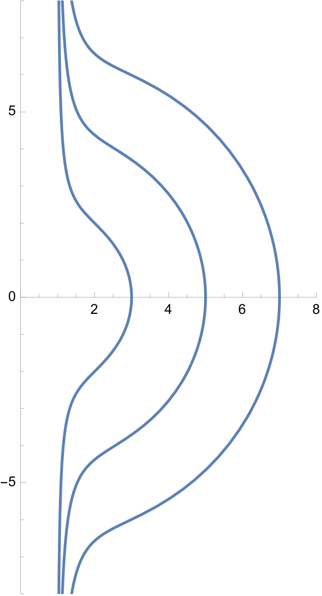
In order to find the family of curves with the properties we wanted, we defined another family of curves, this one with a non-polynomial component (due to substitutions made earlier, this is equivalent to a non-periodic solution). These solutions are of the form $v(z) = tan^{-1}(z)w(z) + g(z)$ where $w(z)$ is one of the previously found polynomials and $g(z)$ is also a polynomial. As a brief note, this is one of my independent contributions: I proved that all the coefficients of $g(z)$ are positive. Some $v(z)$ are displayed below:

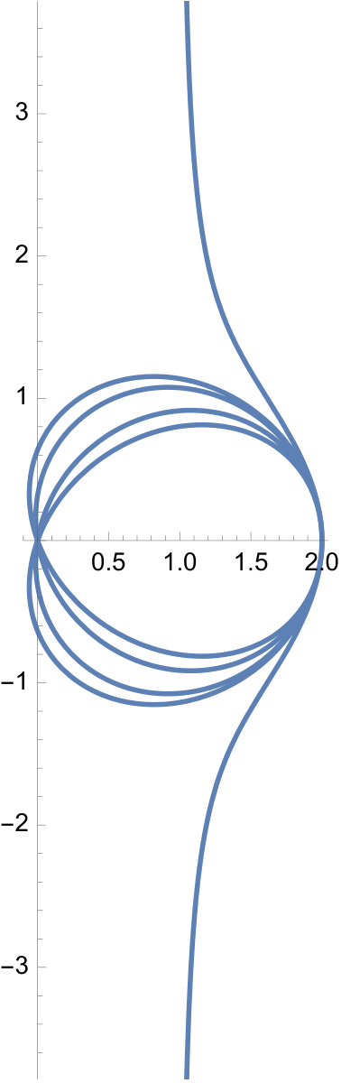
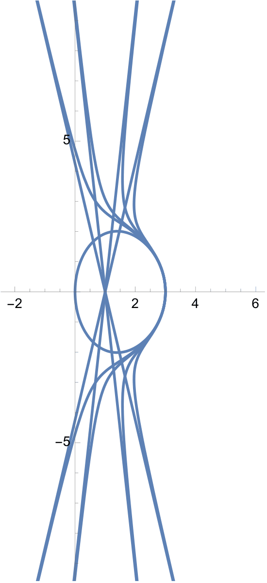
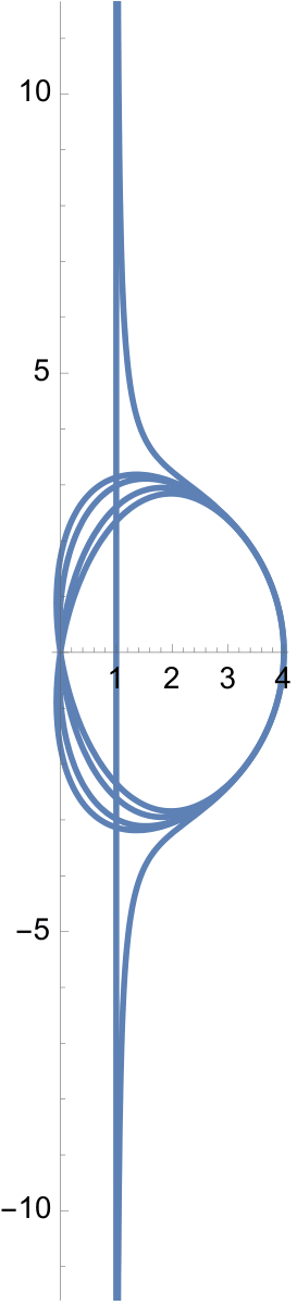
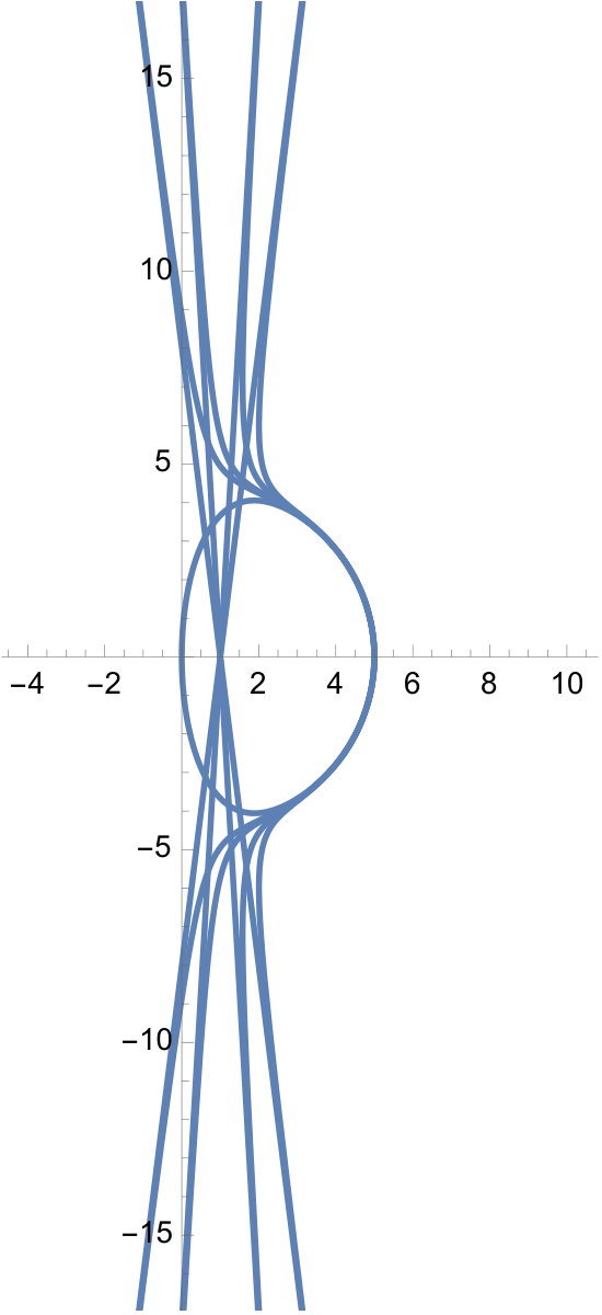
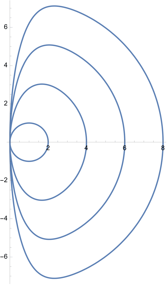
We combined these two families linearly to form a general solution to the differential equations listed above. As the ratio between the families varies (only the ratio matters, as there is a step in the substitution in which the function divides its derivative, and therefore any absolute scaling is lost), the poles and angle at which it crosses the equant vary as well. When this angle is made horizontal, our desired family is revealed:

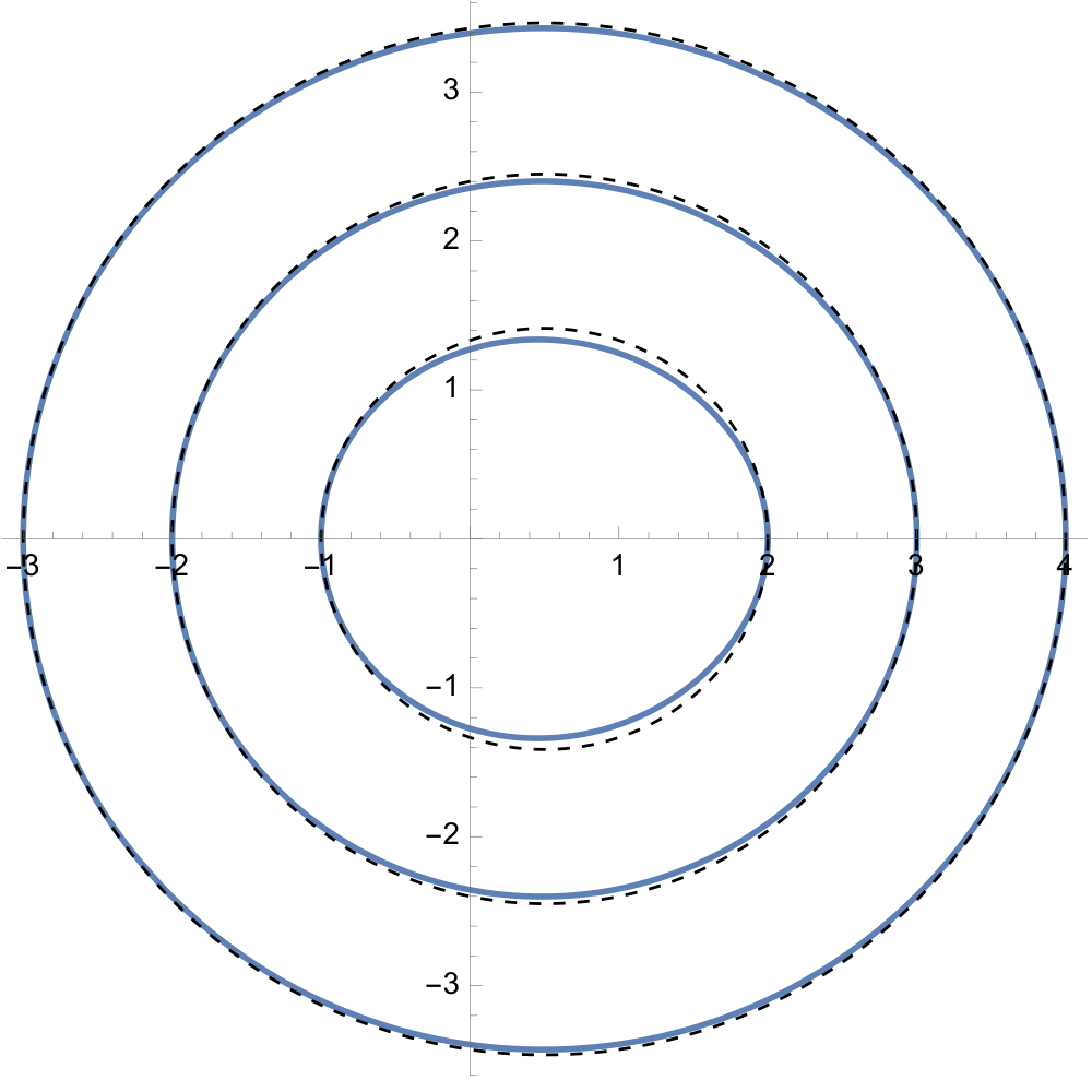
The dashed lines in the above figure represent the ellipses with the same foci, perihelion, and aphelion as the Kepler-Ptolemy curve.

This family has two important limiting characteristics: firstly, it is discrete due to both the other families being discrete and the case that produces the loop family happens only once per polynomial of the form $w(z)$. Secondly, it is not periodic; if extended past $\theta=2\pi$ or before $\theta=0$, it will converge to a periodic solution.

Takeaways:

This project was incredibly instructive, both in the specific subject matter and in general in paper writing and problem-solving skills. I learned:

• New ways of thinking about differential equations
• New methods of substitution for differential equations
• How to use LaTeX (not mentioned previously, but used throughout the paper and this post)
• What Legendre polynomials are and how orthogonality is a useful property
• The general definition of an inner product
• Many other, smaller bits of useful math

I’m very glad to have gotten to learn from Cris on this, and hope to include more projects with him in the future!