Kepler Ptolmey System

This project has spanned over a year and will culminate in the publication of a academic paper in a scientific journal. The subject matter is highly arcane and theoretical, but it has been highly instructive in a variety of areas of mathematics. I am working on this project under the mentorship of Proffessor Cristopher Moore, a researcher at the Santa Fe Institute.

Setup:

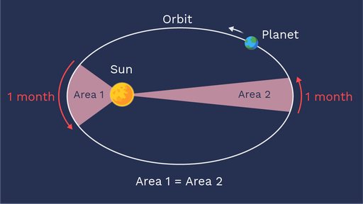
To outline what this project accomplished, I must first discuss certain properties of ellipses, specfically those traced out by one body orbiting another in Newtonian mechanics. In this, angular momentum is conserved from the perspective of the star (which sits at one of the foci), which is an equivalent statement to saying the planet sweeps out equal arcs of area in equal time, as seen in the diagram below.

Another seemingly interesting property of this ellipse is that from the other focus (called the empty focus, because there’s nothing there in a regular orbit) the planet almost conserves its angular speed. This means, standing at that point, the planet would sweep out very close to equal arcs of the sky per unit time.

Proving that in and of itself involved a non-trivial amount of work. I learned to use Mathematica, a software that can be extremely helpful for any sort of complex mathematics. I also gained a much more thorough understanding of variance, which is what we used to quantify the error from a uniform angular speed. As it turned out, the variance was proportional to a forth-order term in the eccentricity of the ellipse, ε. As such, for low eccentricities, uniform angular speed is a very good approxiamtion.

The main problem we addressed, however, was finding a curve which exactly satisfies both the constant angular speed from one focus (which is just what we called them due to their correspondance to the foci of an ellipse - it doesn’t have any of the other properties of ellipse foci) and constant angular momentum from the other.

Main problem:

To address this problem, it needs to be rephrased. The terminology used will be as follows:

\[\vec{r} \text{ is the radius from the empty focus to the planet} \\ \vec{v} \{ is the velocity of the planet} \theta \text{ is the angle of the planet from the empty focus} \\ (x, y) \text{ are the cartesian coordinates of the planet, treating the empty focus as the origin} \\ \ell \text{ is the distance between the foci} \\ \vec{r}_\odot = \vec{r} - \vec{\ell} \text{ is the radius from the sun to the planet} \\ \theta_\odot \text{ is the angle of the planet from the sun} \\ \omega \text{ is the angular speed around the empty focus} \\ J \text{ is the angular momentum around the sun focus} \\\]

Now, the two conditions can be specified:

\[\text{Angular speed: }\omega = \frac{\vec{r} \times \vec{v}}{r^2} \\ \text{Angular momentum: }J = \vec{r}_\odot \times \vec{v}\]

From these, we learned several things. Most importantly, $y’ = \frac{\omega r^2 - J}{\ell} $, which we used later as a basis for substitution and conversion to polar coordinates. I won’t go into all the details (I’ll attach a copy of the paper at the bottom which has everything laid out explicitly), but this system of differential equations turns out to be closely related to the Legendre polynomials, which lead to various families of solutions in a process outlined below.